Neural-Backed Decision Trees (NBDTs)
NBDTs are a method to jointly improve both accuracy and interpretability of neural networks, by creating a decision tree from an already trained model - and fine tuning it.
NBDTs can be summarized into 3 different parts:
- Induced Hierarchy
- Tree Supervision Loss
- Fine-tuning model
Induced Hierarchy
An induced hierarchy is a hierarchy built from the weight vector of a model's final fully connected layer. This idea here is that each dimension
within the vector represents a class. Using agglomerative clustering, we can iteratively pair each class together, framing the decisions a model makes
as a binary split (though this is not always the case, hence this is a limitation of this approach). This allows for more model interpretation by
gaining the ability to ascertain which classes are more likely to be paired together.
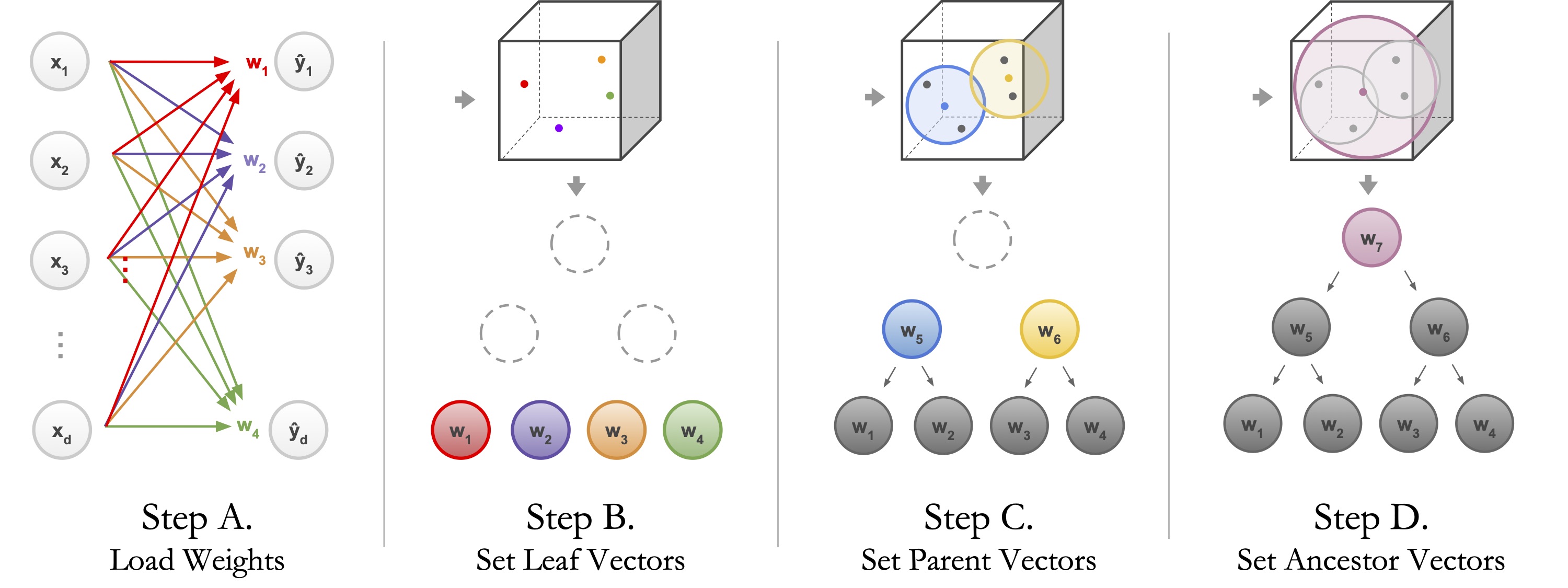
The induced hierarchy tree is produced by first loading the weights of a pre-trained model’s final fully connected layer,
with weight matrix W ∈ R D×K. Then it takes rows ωk ∈ W and normalizes for each leaf node’s weight and averages each pair of leaf nodes for the parents’
weight. Last but not least, for each ancestor, it averages all leaf node weights in its subtree.
That average is the ancestor’s weight. Here, the ancestor is the root, so its weight is the average of all leaf weights ω1, ω2, ω3, ω4.
Tree Supervision Loss
Now, to tune the model, first we have to define a new loss function that can utilize the decision tree structure from the induced hierarchy. We do this by choosing between either Hard or Soft loss, which is defined below.
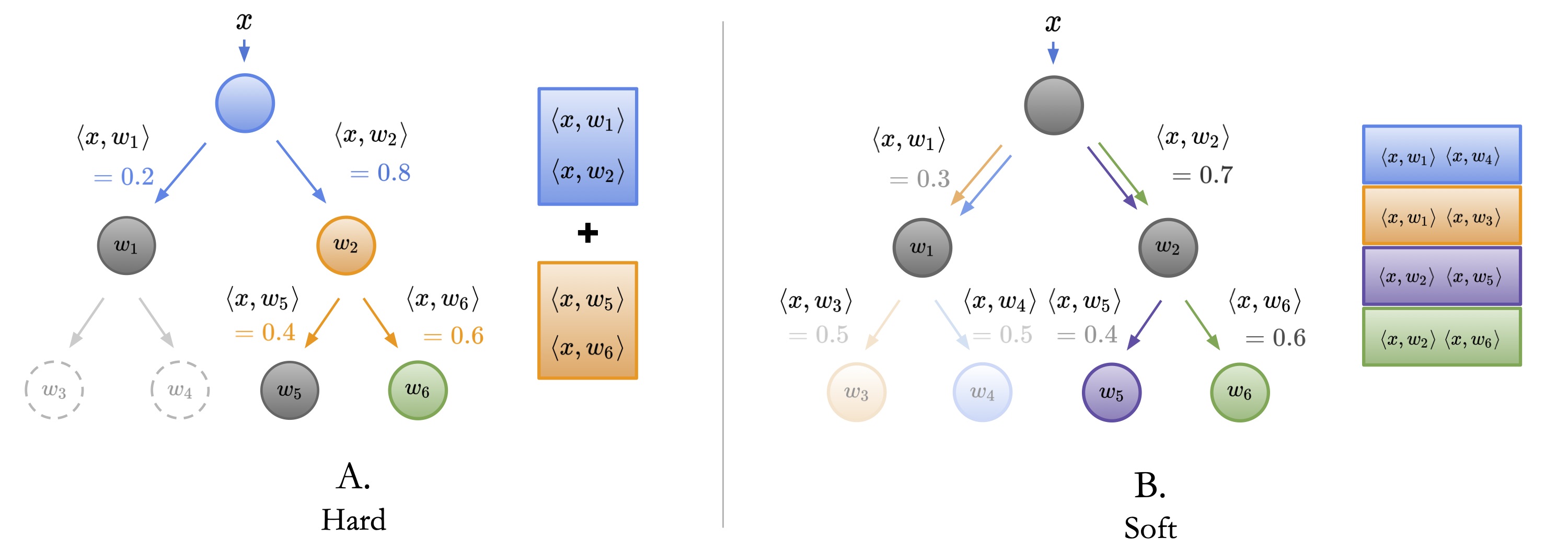
- Hard: is the classic “hard” oblique decision tree. Each node picks the child node with the largest inner product, and visits that node next. Continue until a leaf is reached.
- Soft: is the “soft” variant, where each node simply returns probabilities, as normalized inner products, of each child. For each leaf, compute the probability of its path to the root. Pick leaf with the highest probability.
- Hard vs. Soft: Assume ω4 is the correct class. With hard inference, the mistake at the root (red) is irrecoverable. However, with soft inference, the highly-uncertain decisions at the root and at ω2 are superseded by the highly certain decision at ω3 (green). This means the model can still correctly pick ω4 despite a mistake at the root. In short, soft inference can tolerate mistakes in highly uncertain decisions.
Fine-tuning model
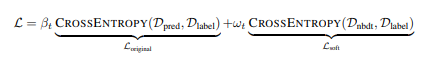
To fine tune the model, we wrap a loss function, in this case CrossEntropyLoss, with ωt and βt being the weights of the original model and the weights of the soft or hard tree loss. Δ here are the probability distributions of the predictions and the labels.